二、在DataFrame中创建新的特性和列

1.导入pandas和matplotlib.pyplot

import pandas as pd
import matplotlib.pyplot as plt
%matplotlib inline

2.读取facebook.csv数据，并设置第一列为索引

fb = pd.read_csv('data/facebook.csv',index_col=0)
ms = pd.read_csv('data/microsoft.csv',index_col=0)
fb.index=pd.to_datetime(fb.index)
ms.index=pd.to_datetime(ms.index)

3.在DataFrame(1)中创建一个新列-差价

#在数据框架fb中创建一个新的列PriceDiff
fb['PriceDiff'] = fb['Close'].shift(-1) - fb['Close']
ms['PriceDiff'] = ms['Close'].shift(-1) - ms['Close']

#运行此代码显示微软在2015-01-05的价差
print(ms['PriceDiff'].loc['2015-01-05'])

Expected Output: -0.68

4.在DataFrame(2)中创建一个新列-每日返回

每日回报按价格/收盘价计算

fb['Return'] = fb['PriceDiff'] /fb['Close']
ms['Return'] = ms['PriceDiff'] /ms['Close']

#运行这段代码打印2015-01-05的返回值
print(ms['Return'].loc['2015-01-05'])

Expected Output: -0.0146773142811

5.使用列表推导-方向在数据框中创建一个新列

# 创建新的列方向。
# List Comprehension的意思是:如果价差大于0，记为1，否则记为0;
#对于DataFrame中的每条记录- fb
fb['Direction'] = [1 if fb['PriceDiff'].loc[ei] > 0 else 0 for ei in fb.index ]
ms['Direction'] = [1 if ms['PriceDiff'].loc[ei] > 0 else 0 for ei in ms.index ]

#运行以下代码显示2015-01-05的价格差异
print('Price difference on {} is {}. direction is {}'.format('2015-01-05', ms['PriceDiff'].loc['2015-01-05'], ms['Direction'].loc['2015-01-05']))

Expected Output: Price difference on 2015-01-05 is -0.6799999999999997. direction is 0

6.使用滚动窗口计算(.rolling()) -移动平均在DataFrame中创建一个新列

fb['ma50'] = fb['Close'].rolling(50).mean()

#绘制移动平均线
plt.figure(figsize=(10, 8))
fb['ma50'].loc['2015-01-01':'2015-12-31'].plot(label='MA50')
fb['Close'].loc['2015-01-01':'2015-12-31'].plot(label='Close')
plt.margins(x=0)
plt.legend()
plt.show()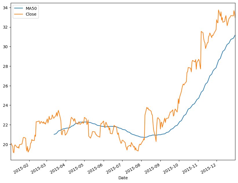

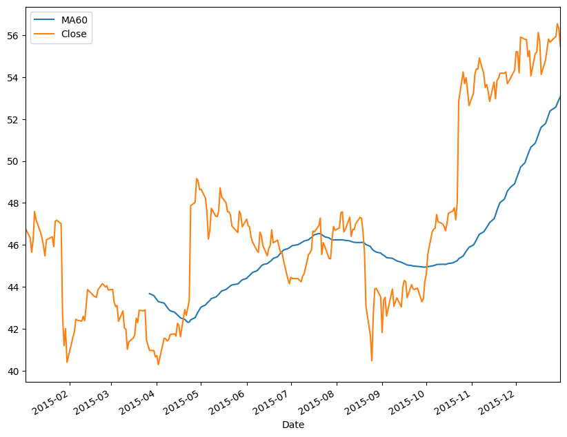
#你可以使用.rolling()来计算任意天数的移动平均线。现在轮到你计算“60天”了
#微软移动平均线，重命名为“ma60”。按照上面的代码绘制图表
ms['ma60'] = ms['Close'].rolling(60).mean()

#绘制移动平均线
plt.figure(figsize=(10, 8))
ms['ma60'].loc['2015-01-01':'2015-12-31'].plot(label='MA60')
ms['Close'].loc['2015-01-01':'2015-12-31'].plot(label='Close')
plt.margins(x=0)
plt.legend()
plt.show()