十二、多元线性回归模型

让我们以不同股票市场的历史数据为基础，模拟构建SPY交易模型的过程

import pandas as pd
import statsmodels.formula.api as smf
import numpy as np
import matplotlib.pyplot as plt
%matplotlib inline
import warnings
warnings.filterwarnings("ignore")
# import all stock market data into DataFrame
aord = pd.read_csv('data/indice/ALLOrdinary.csv')
nikkei = pd.read_csv('data/indice/Nikkei225.csv')
hsi = pd.read_csv('data/indice/HSI.csv')
daxi = pd.read_csv('data/indice/DAXI.csv')
cac40 = pd.read_csv('data/indice/CAC40.csv')
sp500 = pd.read_csv('data/indice/SP500.csv')
dji = pd.read_csv('data/indice/DJI.csv')
nasdaq = pd.read_csv('data/indice/nasdaq_composite.csv')
spy = pd.read_csv('data/indice/SPY.csv')
nasdaq.head()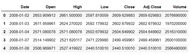

Step 1: Data Munging

# Due to the timezone issues, we extract and calculate appropriate stock market data for analysis
# Indicepanel is the DataFrame of our trading model
indicepanel=pd.DataFrame(index=spy.index)

indicepanel['spy']=spy['Open'].shift(-1)-spy['Open']
indicepanel['spy_lag1']=indicepanel['spy'].shift(1)
indicepanel['sp500']=sp500["Open"]-sp500['Open'].shift(1)
indicepanel['nasdaq']=nasdaq['Open']-nasdaq['Open'].shift(1)
indicepanel['dji']=dji['Open']-dji['Open'].shift(1)

indicepanel['cac40']=cac40['Open']-cac40['Open'].shift(1)
indicepanel['daxi']=daxi['Open']-daxi['Open'].shift(1)

indicepanel['aord']=aord['Close']-aord['Open']
indicepanel['hsi']=hsi['Close']-hsi['Open']
indicepanel['nikkei']=nikkei['Close']-nikkei['Open']
indicepanel['Price']=spy['Open']
indicepanel.head()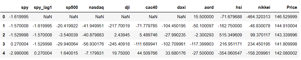

# Lets check whether do we have NaN values in indicepanel
indicepanel.isnull().sum()

spy 1
spy_lag1 1
sp500 1
nasdaq 1
dji 1
cac40 3
daxi 11
aord 2
hsi 57
nikkei 57
Price 0
dtype: int64

# We can use method 'fillna()' from dataframe to forward filling the Nan values
# Then we can drop the reminding Nan values
indicepanel = indicepanel.fillna(method='ffill')
indicepanel = indicepanel.dropna()
# Lets check whether do we have Nan values in indicepanel now
indicepanel.isnull().sum()

spy 0
spy_lag1 0
sp500 0
nasdaq 0
dji 0
cac40 0
daxi 0
aord 0
hsi 0
nikkei 0
Price 0
dtype: int64

# save this indicepanel for part 4.5
path_save = 'data/indice/indicepanel.csv'
indicepanel.to_csv(path_save)
print(indicepanel.shape)

(2678, 11)

Step 2: Data Spliting

#split the data into (1)train set and (2)test set

Train = indicepanel.iloc[-2000:-1000, :]
Test = indicepanel.iloc[-1000:, :]
print(Train.shape, Test.shape)

(1000, 11) (1000, 11)

Step 3: Explore the train data set

# Generate scatter matrix among all stock markets (and the price of SPY) to observe the association

from pandas.plotting import scatter_matrix
sm = scatter_matrix(Train, figsize=(10, 10))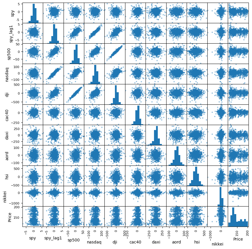

Step 4: Check the correlation of each index between spy

# Find the indice with largest correlation
corr_array = Train.iloc[:, :-1].corr()['spy']
print(corr_array)

spy 1.000000
spy_lag1 -0.011623
sp500 -0.018632
nasdaq 0.012333
dji -0.037097
cac40 0.076886
daxi 0.019410
aord 0.048200
hsi -0.038361
nikkei 0.035379
Name: spy, dtype: float64

formula = 'spy~spy_lag1+sp500+nasdaq+dji+cac40+aord+daxi+nikkei+hsi'
lm = smf.ols(formula=formula, data=Train).fit()
lm.summary()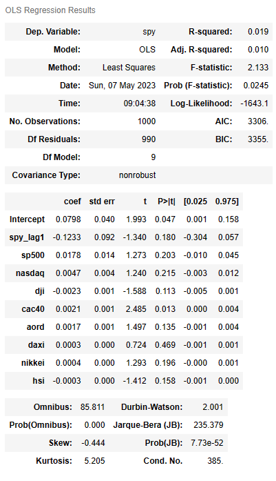

Notes:
[1] Standard Errors assume that the covariance matrix of the errors is correctly specified.

Step 5: Make prediction

Train['PredictedY'] = lm.predict(Train)
Test['PredictedY'] = lm.predict(Test)
plt.scatter(Train['spy'], Train['PredictedY'])

<matplotlib.collections.PathCollection at 0x210353c2a50>

Step 6: Model evaluation - Statistical standard

We can measure the performance of our model using some statistical metrics - RMSE, Adjusted 𝑅2�2

# RMSE - Root Mean Squared Error, Adjusted R^2
def adjustedMetric(data, model, model_k, yname):
    data['yhat'] = model.predict(data)
    SST = ((data[yname] - data[yname].mean())**2).sum()
    SSR = ((data['yhat'] - data[yname].mean())**2).sum()
    SSE = ((data[yname] - data['yhat'])**2).sum()
    r2 = SSR/SST
    adjustR2 = 1 - (1-r2)*(data.shape[0] - 1)/(data.shape[0] -model_k -1)
    RMSE = (SSE/(data.shape[0] -model_k -1))**0.5
    return adjustR2, RMSE
def assessTable(test, train, model, model_k, yname):
    r2test, RMSEtest = adjustedMetric(test, model, model_k, yname)
    r2train, RMSEtrain = adjustedMetric(train, model, model_k, yname)
    assessment = pd.DataFrame(index=['R2', 'RMSE'], columns=['Train', 'Test'])
    assessment['Train'] = [r2train, RMSEtrain]
    assessment['Test'] = [r2test, RMSEtest]
    return assessment
# Get the assement table fo our model
assessTable(Test, Train, lm, 9, 'spy')