十四、模型诊断
小于 1 分钟
import pandas as pd
import statsmodels.formula.api as smf
import matplotlib.pyplot as plt
% matplotlib inline
housing = pd.DataFrame.from_csv('data/housing.csv')
housing.head()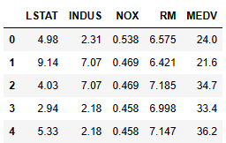
model = smf.ols(formula='MEDV~LSTAT', data=housing).fit()

# Here are estimated intercept and slope by least square estimation
b0_ols = model.params[0]
b1_ols = model.params[1]

housing['BestResponse'] = b0_ols + b1_ols*housing['LSTAT']
Assumptions behind linear regression model
- Linearity
- independence
- Normality
- Equal Variance
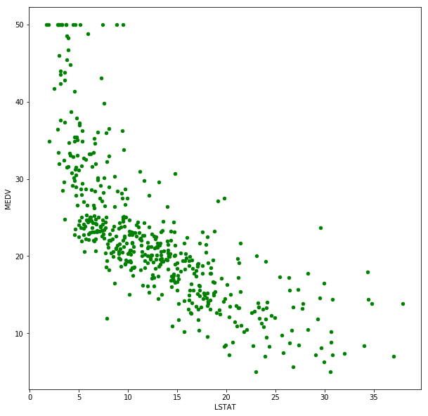
Linearity
# you can check the scatter plot to have a fast check
housing.plot(kind='scatter', x='LSTAT', y='MEDV', figsize=(10, 10), color='g')
<matplotlib.axes._subplots.AxesSubplot at 0x7efdfb538940>
Independence
# Get all errors (residuals)
housing['error'] = housing['MEDV'] - housing['BestResponse']
# Method 1: Residual vs order plot
# error vs order plot (Residual vs order) as a fast check
plt.figure(figsize=(15, 8))
plt.title('Residual vs order')
plt.plot(housing.index, housing['error'], color='purple')
plt.axhline(y=0, color='red')
plt.show()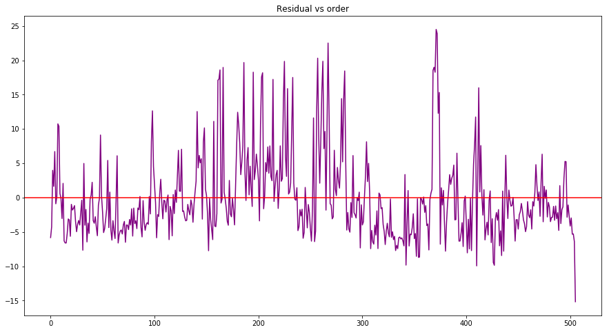
# Method 2: Durbin Watson Test
# Check the Durbin Watson Statistic
# Rule of thumb: test statistic value in the range of 1.5 to 2.5 are relatively normal
model.summary()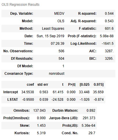
Warnings:
[1] Standard Errors assume that the covariance matrix of the errors is correctly specified.
Normality
import scipy.stats as stats
z = (housing['error'] - housing['error'].mean())/housing['error'].std(ddof=1)

stats.probplot(z, dist='norm', plot=plt)
plt.title('Normal Q-Q plot')
plt.show()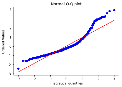
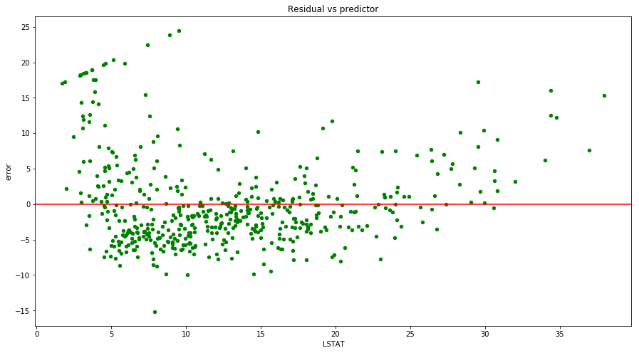
Equal variance
# Residual vs predictor plot
housing.plot(kind='scatter', x='LSTAT', y='error', figsize=(15, 8), color='green')
plt.title('Residual vs predictor')
plt.axhline(y=0, color='red')
plt.show()