十一、简单线性回归模型

import pandas as pd
import statsmodels.formula.api as smf
import matplotlib.pyplot as plt
% matplotlib inline
housing = pd.DataFrame.from_csv('data/housing.csv')
housing.head()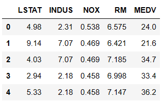

Simple linear regression

We shall base on the association between LSTAT and MEDV and create a simple linear regression model. Let's use python in estimating the values of B0 and B1 (intercept and slope)

# lets try to guess what are the real values of intercept and slope
# we call our guess b0, b1...
# Try to assign the value of b0, b1 to get a straight line that can describe our data 
b0 = 0.1
b1 = 1
housing['GuessResponse'] = b0 + b1*housing['RM']

# Also want to know the error of of guess...
# This show how far is our guess response from the true response
housing['observederror'] = housing['MEDV'] - housing['GuessResponse']


# plot your estimated line together with the points
plt.figure(figsize=(10, 10))
plt.title('Sum of sqaured error is {}'.format((((housing['observederror'])**2)).sum()))
plt.scatter(housing['RM'], housing['MEDV'], color='g', label='Observed')
plt.plot(housing['RM'], housing['GuessResponse'], color='red', label='GuessResponse')
plt.legend()
plt.xlim(housing['RM'].min()-2, housing['RM'].max()+2)
plt.ylim(housing['MEDV'].min()-2, housing['MEDV'].max()+2)
plt.show()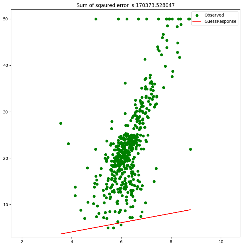

Least sqaure estimates

# Input the formula (refer to the lecture video 4.3)
formula = 'MEDV~RM'
model = smf.ols(formula=formula, data=housing).fit()

# Here are estimated intercept and slope by least square estimation
# Attribute 'params' returns a list of estimated parameters form model
b0_ols = model.params[0]
b1_ols = model.params[1]

housing['BestResponse'] = b0_ols + b1_ols*housing['RM']

# Also want to know the error of of guess...
housing['error'] = housing['MEDV'] - housing['BestResponse']


# plot your estimated line together with the points
plt.figure(figsize=(10, 10))
# See if the error drops after you use least square method
plt.title('Sum of sqaured error is {}'.format((((housing['error'])**2)).sum()))
plt.scatter(housing['RM'], housing['MEDV'], color='g', label='Observed')
plt.plot(housing['RM'], housing['GuessResponse'], color='red', label='GuessResponse')
plt.plot(housing['RM'], housing['BestResponse'], color='yellow', label='BestResponse')
plt.legend()
plt.xlim(housing['RM'].min()-2, housing['RM'].max()+2)
plt.ylim(housing['MEDV'].min()-2, housing['MEDV'].max()+2)
plt.show()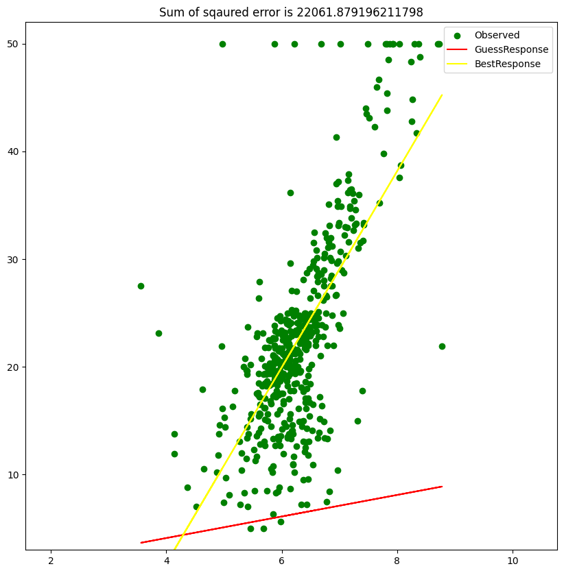

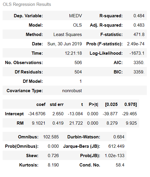
Summary table

#Refer to the P-value of RM, Confidence Interval and R-square to evaluate the performance.
model.summary()