十三、基于回归模型的评估策略

import statsmodels.formula.api as smf
import pandas as pd
import numpy as np
import matplotlib.pyplot as plt
%matplotlib inline
import warnings
warnings.filterwarnings("ignore")
indicepanel = pd.read_csv('data/indice/indicepanel.csv')
indicepanel.head()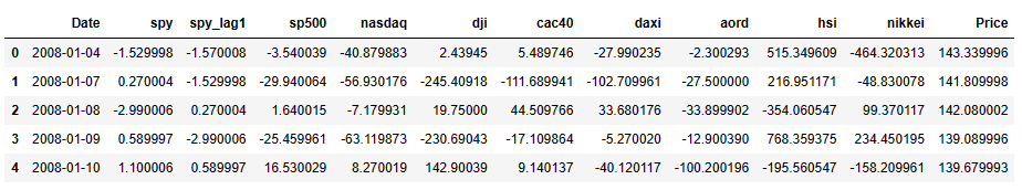

Train = indicepanel.iloc[-2000:-1000, :]
Test = indicepanel.iloc[-1000:, :]
formula = 'spy~spy_lag1+sp500+nasdaq+dji+cac40+aord+daxi+nikkei+hsi'
lm = smf.ols(formula=formula, data=Train).fit()
Train['PredictedY'] = lm.predict(Train)
Test['PredictedY'] = lm.predict(Test)

Profit of Signal-based strategy

# Train
Train['Order'] = [1 if sig>0 else -1 for sig in Train['PredictedY']]
Train['Profit'] = Train['spy'] * Train['Order']

Train['Wealth'] = Train['Profit'].cumsum()
print('Total profit made in Train: ', Train['Profit'].sum())

Total profit made in Train: 214.34009500000042

plt.figure(figsize=(10, 10))
plt.title('Performance of Strategy in Train')
plt.plot(Train['Wealth'].values, color='green', label='Signal based strategy')
plt.plot(Train['spy'].cumsum().values, color='red', label='Buy and Hold strategy')
plt.legend()
plt.show()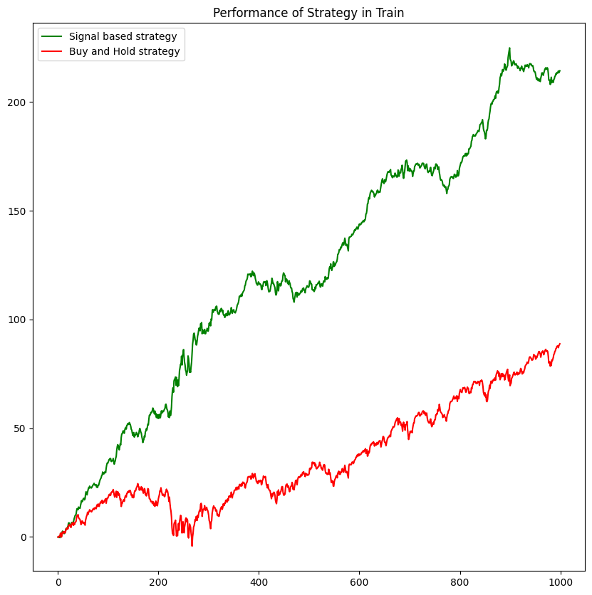

# Test
Test['Order'] = [1 if sig>0 else -1 for sig in Test['PredictedY']]
Test['Profit'] = Test['spy'] * Test['Order']

Test['Wealth'] = Test['Profit'].cumsum()
print('Total profit made in Test: ', Test['Profit'].sum())

Total profit made in Test: 241.0300879999996

plt.figure(figsize=(10, 10))
plt.title('Performance of Strategy in Train')
plt.plot(Test['Wealth'].values, color='green', label='Signal based strategy')
plt.plot(Test['spy'].cumsum().values, color='red', label='Buy and Hold strategy')
plt.legend()
plt.show()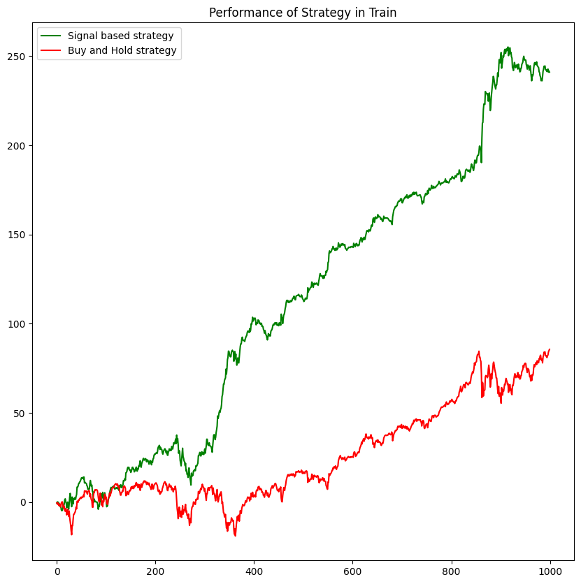

Evaluation of model - Practical Standard

We introduce two common practical standards - Sharpe Ratio, Maximum Drawdown to evaluate our model performance

Train['Wealth'] = Train['Wealth'] + Train.loc[Train.index[0], 'Price']
Test['Wealth'] = Test['Wealth'] + Test.loc[Test.index[0], 'Price']
# Sharpe Ratio on Train data
Train['Return'] = np.log(Train['Wealth']) - np.log(Train['Wealth'].shift(1))
dailyr = Train['Return'].dropna()

print('Daily Sharpe Ratio is ', dailyr.mean()/dailyr.std(ddof=1))
print('Yearly Sharpe Ratio is ', (252**0.5)*dailyr.mean()/dailyr.std(ddof=1))

Daily Sharpe Ratio is 0.17965076303258012
Yearly Sharpe Ratio is 2.851867450963218

# Sharpe Ratio in Test data
Test['Return'] = np.log(Test['Wealth']) - np.log(Test['Wealth'].shift(1))
dailyr = Test['Return'].dropna()

print('Daily Sharpe Ratio is ', dailyr.mean()/dailyr.std(ddof=1))
print('Yearly Sharpe Ratio is ', (252**0.5)*dailyr.mean()/dailyr.std(ddof=1))

Daily Sharpe Ratio is 0.13035126208575046
Yearly Sharpe Ratio is 2.06926213537379

# Maximum Drawdown in Train data
Train['Peak'] = Train['Wealth'].cummax()
Train['Drawdown'] = (Train['Peak'] - Train['Wealth'])/Train['Peak']
print('Maximum Drawdown in Train is ', Train['Drawdown'].max())

Maximum Drawdown in Train is 0.06069016443644383

# Maximum Drawdown in Test data
Test['Peak'] = Test['Wealth'].cummax()
Test['Drawdown'] = (Test['Peak'] - Test['Wealth'])/Test['Peak']
print('Maximum Drawdown in Test is ', Test['Drawdown'].max())

Maximum Drawdown in Test is 0.11719899524631659